Sparse Table

I’m excited to present Sparse Tables. Despite being somewhat niche, Sparse Tables are simple to implement and extremely powerful.

The Problem

Let’s suppose:

we have an array a of some type
we have some associative binary function f ^[*]. The function can be: min, max, gcd, boolean AND, boolean OR …

^[*] where f is also “idempotent”. Don’t worry, I’ll explain this in a moment.

Our task is as follows:

Given two indices l and r, answer a query for the interval [l, r) by performing f(a[l], a[l + 1], a[l + 2], ..., a[r - 1]); taking all the elements in the range and applying f to them
There will be a huge number Q of these queries to answer … so we should be able to answer each query quickly!

For example, if we have an array of numbers:

var a = [ 20, 3, -1, 101, 14, 29, 5, 61, 99 ]

and our function f is the min function.

Then we may be given a query for interval [3, 8). That means we look at the elements:

101, 14, 29, 5, 61

because these are the elements of a with indices that lie in our range [3, 8) – elements from index 3 up to, but not including, index 8. We then we pass all of these numbers into the min function, which takes the minimum. The answer to the query is 5, because that’s the result of min(101, 14, 29, 5, 61).

Imagine we have millions of these queries to process.

Query 1: Find minimum of all elements between 2 and 5

Query 2: Find minimum of all elements between 3 and 9

…

Query 1000000: Find minimum of all elements between 1 and 4

And our array is very large. Here, let’s say Q = 1000000 and N = 500000. Both numbers are huge. We want to make sure that we can answer each query really quickly, or else the number of queries will overwhelm us!

So that’s the problem.

The naive solution to this problem is to perform a for loop to compute the answer for each query. However, for very large Q and very large N this will be too slow. We can speed up the time to compute the answer by using a data structure called a Sparse Table. You’ll notice that so far, our problem is exactly the same as that of the Segment Tree (assuming you’re familiar). However! … there’s one crucial difference between Segment Trees and Sparse Tables … and it concerns our choice of f.

A small gotcha … Idempotency

Suppose we wanted to find the answer to [A, D). And we already know the answer to two ranges [A, B) and [C, D). And importantly here, … these ranges overlap!! We have C < B.

Overlapping ranges

So what? Well, for f = minimum function, we can take our answers for [A, B) and [C, D) and combine them! We can just take the minimum of the two answers: result = min(x1, x2) … voilà!, we have the minimum for [A, D). It didn’t matter that the intervals overlap - we still found the correct minimum. But now suppose f is the addition operation +. Ok, so now we’re taking sums over ranges. If we tried the same approach again, it wouldn’t work. That is, if we took our answers for [A, B) and [C, D) and added them together we’d get a wrong answer for [A, D). Why? Well, we’d have counted some elements twice because of the overlap.

Later, we’ll see that in order to answer queries, Sparse Tables use this very technique. They combine answers in the same way as shown above. Unfortunately this means we have to exclude certain binary operators from being f, including +, *, XOR, … because they don’t work with this technique. In order to get the best speed of a Sparse Table, we need to make sure that the f we’re using is an idempotent binary operator. Mathematically, these are operators that satisfy f(x, x) = x for all possible x that could be in a. Practically speaking, these are the only operators that work; allowing us to combine answers from overlapping ranges. Examples of idempotent f’s are min, max, gcd, boolean AND, boolean OR, bitwise AND and bitwise OR. Note that for Segment Trees, f does not have to be idempotent. That’s the crucial difference between Segment Trees and Sparse Tables.

Phew! Now that we’ve got that out of the way, let’s dive in!

Structure of a Sparse Table

Let’s use f = min and use the array:

var a = [ 10, 6, 5, -7, 9, -8, 2, 4, 20 ]

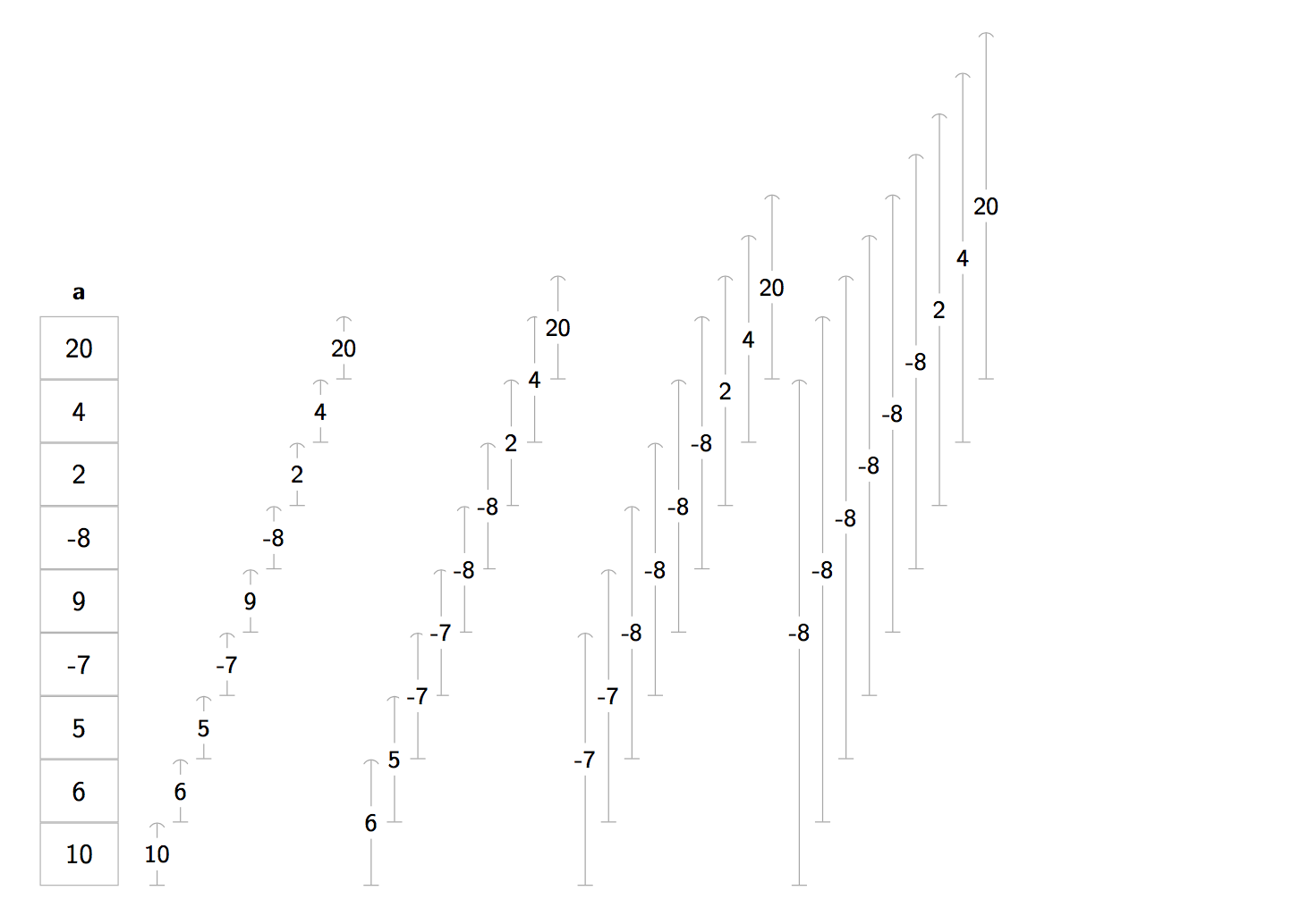
In this case, the Sparse Table looks like this:

Sparse Table

What’s going on here? There seems to be loads of intervals. Correct! Sparse tables are preloaded with the answers for lots of queries [l, r). Here’s the idea. Before we process our Q queries, we’ll pre-populate our Sparse Table table with answers to loads of queries; making it act a bit like a cache. When we come to answer one of our queries, we can break the query down into smaller “sub-queries”, each having an answer that’s already in the cache. We lookup the cached answers for the sub-queries in table in constant time and combine the answers together to give the overall answer to the original query in speedy time.

The problem is, we can’t store the answers for every single possible query that we could ever have … or else our table would be too big! After all, our Sparse Table needs to be sparse. So what do we do? We only pick the “best” intervals to store answers for. And as it turns out, the “best” intervals are those that have a width that is a power of two!

For example, the answer for the query [10, 18) is in our table because the interval width: 18 - 10 = 8 = 2**3 is a power of two (** is the exponentiation operator). Also, the answer for [15, 31) is in our table because its width: 31 - 15 = 16 = 2**4 is again a power of two. However, the answer for [1, 6) is not in there because the interval’s width: 6 - 1 = 5 is not a power of two. Consequently, we don’t store answers for all possible intervals that fit inside a – only the ones with a width that is a power of two. This is true irrespective of where the interval starts within a. We’ll gradually see that this approach works and that relatively speaking, it uses very little space.

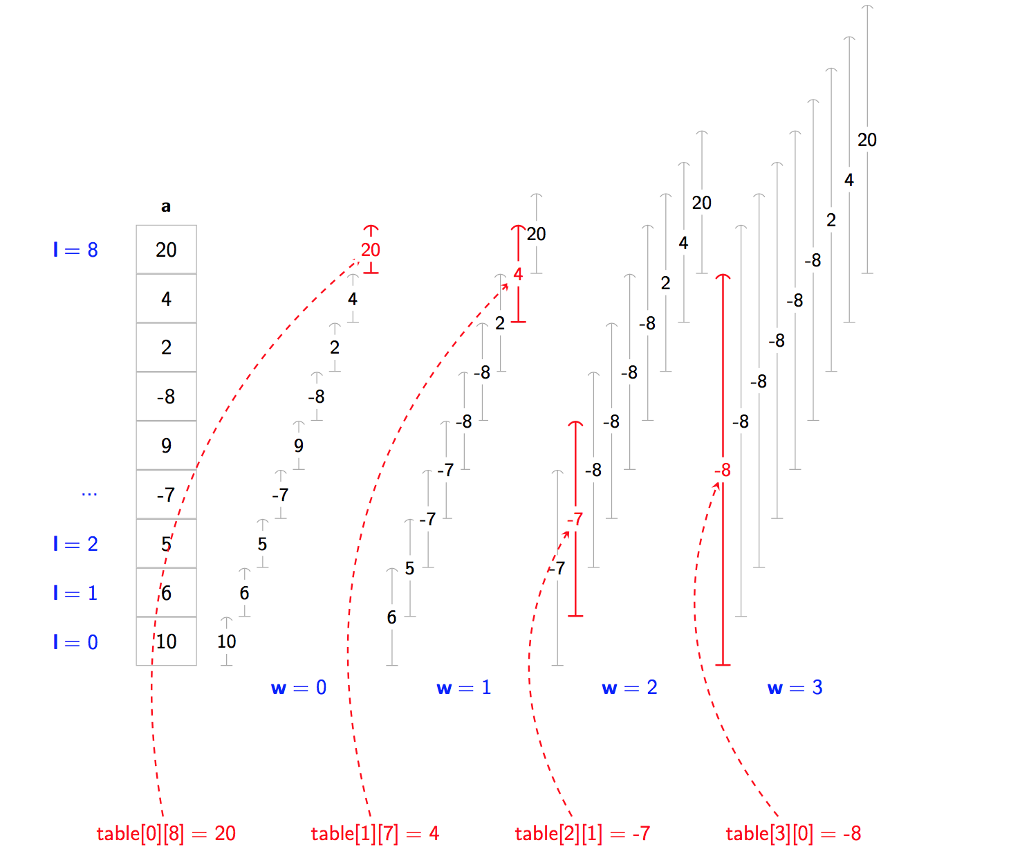
A Sparse Table is a table where table[w][l] contains the answer for [l, l + 2**w).
It has entries table[w][l] where:

w tells us our width … the number of elements or the width is 2**w
l tells us the lower bound … it’s the starting point of our interval

Some examples:

table[3][0] = -8: our width is 2**3, we start at l = 0 so our query is [0, 0 + 2**3) = [0, 8).
The answer for this query is min(10, 6, 5, -7, 9, -8, 2, 4, 20) = -8.
table[2][1] = -7: our width is 2**2, we start at l = 1 so our query is [1, 1 + 2**2) = [1, 5).
The answer for this query is min(6, 5, -7, 9) = -7.
table[1][7] = 4: our width is 2**1, we start at l = 7 so our query is [7, 7 + 2**1) = [7, 9).
The answer for this query is min(4, 20) = 4.
table[0][8] = 20: our width is 2**0, we start at l = 8 so our query is[8, 8 + 2**0) = [8, 9).
The answer for this query is min(20) = 20.

Sparse Table

A Sparse Table can be implemented using a two-dimentional array.

public class SparseTable<T> {
  private var table: [[T]]

  public init(array: [T], function: @escaping (T, T) -> T, defaultT: T) {
      table = [[T]](repeating: [T](repeating: defaultT, count: N), count: W)
  }
  // ...    
}

Building a Sparse Table

To build a Sparse Table, we compute each table entry starting from the bottom-left and moving up towards the top-right (in accordance with the diagram). First we’ll compute all the intervals for w = 0, then compute all the intervals and for w = 1 and so on. We’ll continue up until w is big enough such that our intervals are can cover at least half the array. For each w, we compute the interval for l = 0, 1, 2, 3, … until we reach N. This is all achieved using a double for-in loop:

for w in 0..<W {
  for l in 0..<N {
    // compute table[w][l]
  }
}

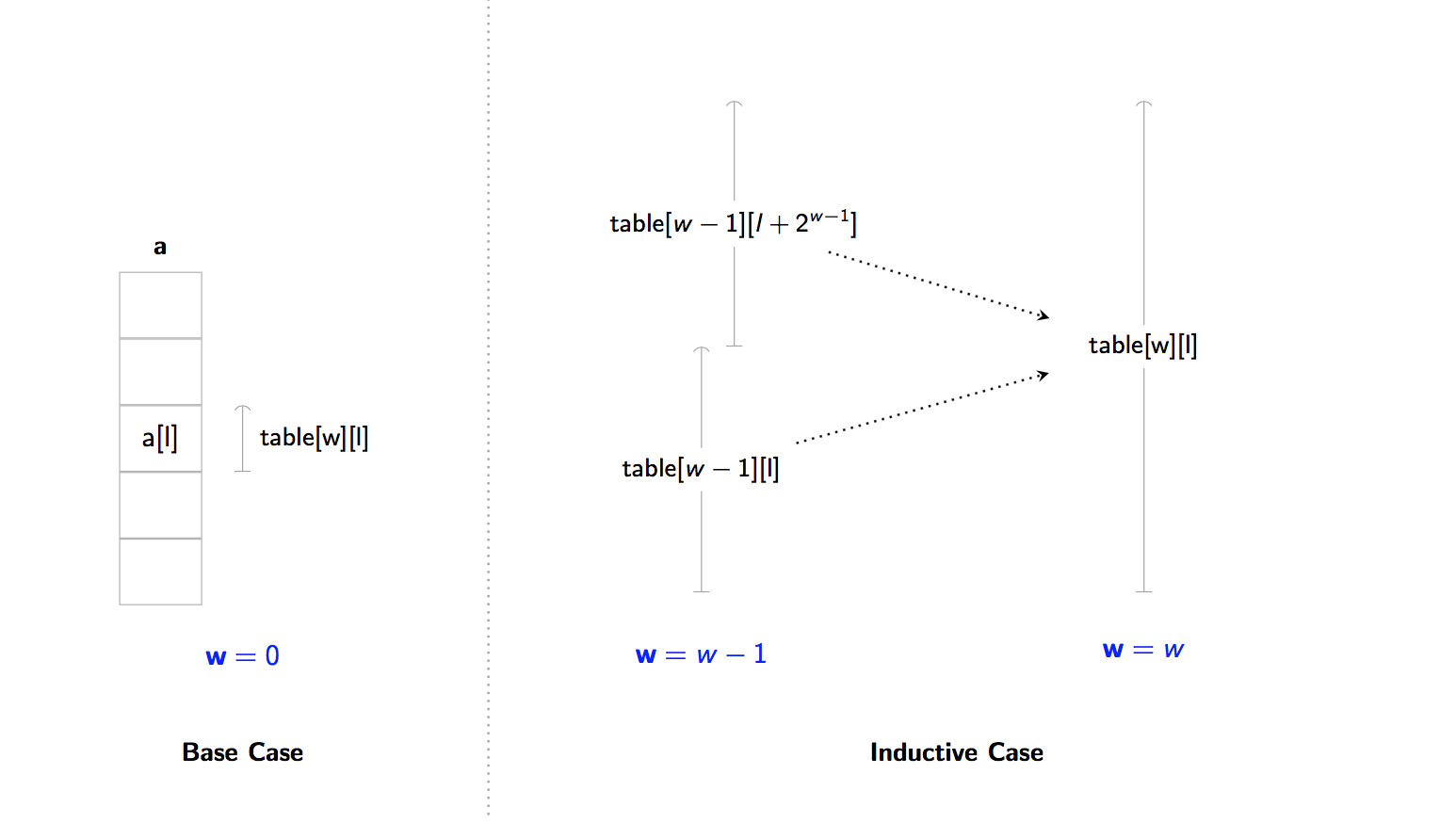
To compute table[w][l]:

Base Case (w = 0): Each interval has width 2**w = 1.
- We have one element intervals of the form: [l, l + 1).
- The answer is just a[l] (e.g. the minimum of over a list with one element is just the element itself).
```
table[w][l] = a[l]
```
Inductive Case (w > 0): We need to find out the answer to [l, l + 2**w) for some l. This interval, like all of our intervals in our table has a width that is a power of two (e.g. 2, 4, 8, 16) … so we can cut it into two equal halves.
- Our interval with width 2**w is cut into two intervals, each of width 2**(w - 1).
- Because each half has a width that is a power of two, we can look them up in our Sparse Table.
- We combine them together using f.
```
  table[w][l] = f(table[w - 1][l], table[w - 1][l + 2 ** (w - 1)])
```

Sparse Table

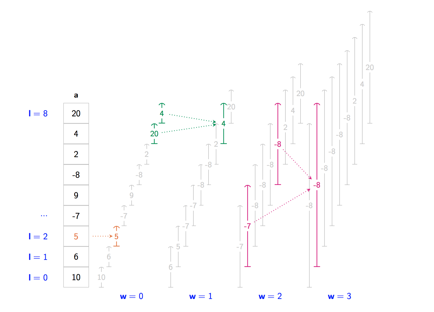
For example for a = [ 10, 6, 5, -7, 9, -8, 2, 4, 20 ] and f = min:

we compute table[0][2] = 5. We just had to look at a[2] because the range has a width of one.
we compute table[1][7] = 4. We looked at table[0][7] and table[0][8] and apply f to them.
we compute table[3][1] = -8. We looked at table[2][1] and table[2][5] and apply f to them.

Sparse Table

public init(array: [T], function: @escaping (T, T) -> T, defaultT: T) {
 let N = array.count
 let W = Int(ceil(log2(Double(N))))
 table = [[T]](repeating: [T](repeating: defaultT, count: N), count: W)
 self.function = function
 self.defaultT = defaultT

 for w in 0..<W {
   for l in 0..<N {
     if w == 0 {
       table[w][l] = array[l]
     } else {
       let first = self.table[w - 1][l]
       let secondIndex = l + (1 << (w - 1))
       let second = ((0..<N).contains(secondIndex)) ? table[w - 1][secondIndex] : defaultT
       table[w][l] = function(first, second)
     }
   }
 }
}

Building a Sparse Table takes O(NlogN) time.
The table itself uses O(NlgN) additional space.

Getting Answers to Queries

Suppose we’ve built our Sparse Table. And now we’re going to process our Q queries. Here’s where our work pays off.

Let’s suppose f = min and we have:

var a = [ 10, 6, 5, -7, 9, -8, 2, 4, 20 ]

And we have a query [3, 9).

First let’s find the largest power of two that fits inside [3, 9). Our interval has width 9 - 3 = 6. So the largest power of two that fits inside is four.
We create two new queries of [3, 7) and [5, 9) that have a width of four. And, we arrange them so that to that they span the whole interval without leaving any gaps.
Because these two intervals have a width that is exactly a power of two we can lookup their answers in the Sparse Table using the entries for w = 2. The answer to [3, 7) is given by table[2][3], and the answer to [5, 9) is given by table[2][5]. We compute and return min(table[2][3], table[2][5]). This is our final answer! :tada:. Although the two intervals overlap, it doesn’t matter because the f = min we originally chose is idempotent.

In general, for each query: [l, r) …

Find W, by looking for the largest width that fits inside the interval that’s also a power of two. Let largest such width = 2**W.
Form two sub-queries of width 2**W and arrange them to that they span the whole interval without leaving gaps. To guarantee there are no gaps, we need to align one half to the left and the align other half to the right.

Compute and return f(table[W][l], table[W][r - 2**W]).

   public func query(from l: Int, until r: Int) -> T {
     let width = r - l
     let W = Int(floor(log2(Double(width))))
     let lo = table[W][l]
     let hi = table[W][r - (1 << W)]
     return function(lo, hi)
  }

Finding answers to queries takes O(1) time.

Analysing Sparse Tables

Query Time - Both table lookups take constant time. All other operations inside query take constant time. So answering a single query also takes constant time: O(1). But instead of one query we’re actually answering Q queries, and we’ll need time to built the table before-hand. Overall time is: O(NlgN + Q) to build the table and answer all queries. The naive approach is to do a for loop for each query. The overall time for the naive approach is: O(NQ). For very large Q, the naive approach will scale poorly. For example if Q = O(N*N) then the naive approach is O(N*N*N) where a Sparse Table takes time O(N*N).
Space- The number of possible w is lgN and the number of possible l our table is N. So the table has uses O(NlgN) additional space.

Comparison with Segment Trees

Pre-processing - Segment Trees take O(N) time to build and use O(N) space. Sparse Tables take O(NlgN) time to build and use O(NlgN) space.
Queries - Segment Tree queries are O(lgN) time for any f (idempotent or not idempotent). Sparse Table queries are O(1) time if f is idempotent and are not supported if f is not idempotent. ^[†]
Replacing Items - Segment Trees allow us to efficiently update an element in a and update the segment tree in O(lgN) time. Sparse Tables do not allow this to be done efficiently. If we were to update an element in a, we’d have to rebuild the Sparse Table all over again in O(NlgN) time.

^[†] Although technically, it’s possible to rewrite the query method to add support for non-idempotent functions. But in doing so, we’d bump up the time up from O(1) to O(lgn), completely defeating the original purpose of Sparse Tables - supporting lightening quick queries. In such a case, we’d be better off using a Segment Tree (or a Fenwick Tree)

Summary

That’s it! See the playground for more examples involving Sparse Tables. You’ll see examples for: min, max, gcd, boolean operators and logical operators.

swift-algorithm-club-cn

Swift 数据结构与算法学院！翻译自https://github.com/raywenderlich/swift-algorithm-club

Sparse Table

The Problem

A small gotcha … Idempotency

Structure of a Sparse Table

Building a Sparse Table

Getting Answers to Queries

Analysing Sparse Tables

Comparison with Segment Trees

Summary

See also